45

HEALTHCARE SERVICES
AND GLOBALISATION

An input-output analysis

José Luis NavarroEspigaresa,b

a  Virgen de las Nieves
University Hospital of Granada

b  University of Granada

Introduction

The health sector has traditionally been closed and nationally focused, but during recent decades this perspective has changed. Examples of the globalisation of health include:

–The increasing mobility of health professionals across borders; for example, the United Kingdom now actively recruits nurses from other countries (Glinos, 2015; Shaffer et al., 2016; Maier and Aiken, 2016; Marchal and Kegels, 2003).

–The increasing mobility of health consumers (people); for example, patients travelling abroad to access medical care (Hazarika, 2010; Hopkins et al., 2010; Whittaker et al., 2010).

–The increasing number of foreign private companies that offer health services and international health insurance schemes (Smith et al., 2009; Pachanee, 2006; Herman, 2009).

–The use of new technologies, such as the Internet, to provide health services across borders and to remote regions within countries (Abbott and Coenen, 2008; Haux, 2006).

46

–The higher disease burden in poor countries that requires a more detailed analysis of global health (in which health risks in both poor and rich countries are seen as having inherently global causes and consequences) (Labonté et al., 2011).

–The growing trade, marketing and investment have important implications for public health, as well as the health effects of global trade agreements (Bettcher et al., 2000).

–Environmental impacts and climate change impacts on health (McMichael, 2013).

–And especially, the fact that health science is more and more a global science based on knowledge. As knowledge becomes more global, the globalisation of medical sciences is an irrefutable fact. Specialised training programs for doctors are increasingly widespread and guarantee rapid dissemination of innovations. The pharmaceutical industry is also responsible for the rapid diffusion of innovations in its field, so that in developed countries knowledge and access to new drugs is guaranteed in a short period of time after their discovery.

The main advances in the knowledge of medical science come mainly through new diagnostic techniques, new surgical techniques, and new drugs. In all three cases, the dissemination of knowledge and, above all, the possibility of universal access is linked to international trade and the process of economic globalisation.

While globalisation affects the institutional, economic, socio-cultural and ecological determinants of population health, the globalisation process is usually considered at the contextual level, influencing health through its more distal and proximal determinants (Huynen et al., 2005). A measure of the globalisation of a health system should include its degree of openness to foreign goods, services, people, ideas and policies. However, the openness of healthcare systems is a significant factor that sometimes limits the domestic economic impact of an eventual increase of expenses in national healthcare systems. For example, the recent widespread use of generic medicines has created new channels of trade at an international level (Rana and Roy, 2015). And, more recently, the potential benefit of biosimilar medicines in Europe, by covering the lack of uniformity across EU nations, 47depends on the requirements for competitive functioning markets (IMS Institute, 2016).

In accordance with the classical input-output model, if there is an increase in final demand for a particular product or service (e.g., healthcare services), we can assume that there will be an increase in the output of that production branch, as producers react to meet the increased demand; this is the direct effect. As these producers increase their output, there will also be an increase in demand on their suppliers, and so on down the supply chain; this is the indirect effect. As a result of the direct and indirect effects, the level of household income throughout the economy will increase as a result of increased employment. A proportion of this increased income will be re-spent on final goods and services; this is the induced effect.

As a consequence of globalisation, world trade and production are increasingly structured around “global value chains” (GVCs). A value chain identifies the full range of activities that firms undertake to bring a product or service from its conception to its end, which is its use by the final consumers. Today, more than half of world manufactured imports are intermediate goods (primary goods, parts and components, and semi-finished products), and more than seventy percent of world services imports are intermediate services (Miroudot et al., 2009). Inter-country input-output tables and a full matrix of bilateral trade flows have been used by OECD to derive data on the value added by each country in the value chain, thus giving a better picture of trade flows related to activities of firms in GVCs.

The inputs imported in the health and social works sector have risen from 3.6% of total output in 1995 to 4.9% in 2011. With regard to the value of intermediate consumption in the health sector, the inputs imported have increased from 10.3% in 1995 to 13.1% in 2011. These increases in participation are consistent with recent studies published on the integration of national productive structures in global value chains. One recent published study about GVCs reveals that on average more than half of the value of exports is made up of products traded in the context of global value chains. For advanced economies, one-third of exports were attributed to imported inputs in 2008–12, up from one-quarter in 1991–95. For low-income economies and emerging market economies other than in Sub-Saharan Africa, the average was 21–22% 48in 2008–12, up from 17–18% in 1991–95 (Dollar and Kidder, 2017). While most studies on GVCs have focused on Asia, Europe shows a comparable if not higher level of participation in GVCs (De Backer and Miroudot, 2013).

An important implication of the new GVC paradigm is that one should look beyond industries to understand trade and production patterns. The GVC literature insists on business functions, which are the activities along the supply chain, such as R&D, procurement, operations, marketing, customer services, etc. Countries tend to specialise in specific business functions involving specific tasks rather than specific industries.

In this scenario dominated by strategies based on global value chains, it is interesting to know the influence of this process on traditional impact analysis. The research question we pose in this paper attempts to understand how the process of globalisation influences domestic effects (direct and indirect) of the final demand for health services.

The objective of this work is to analyse the economic impact of National Health Service expenditures on the whole economy from a global and international perspective. To analyse the impact of globalisation on the openness to foreign goods of healthcare services, we will use the latest set of OECD harmonised national Input-Output Tables. This database presents matrices of inter-industrial flows of goods and services (produced domestically as well as imported) with current prices (USD million) for all OECD countries, covering the years 1995 to 2011. Additionally, we will utilise the OECD’s Inter-Country Input-Output Tables. In those tables, the diagonal blocks represent domestic transaction flows of intermediate goods and services across industries, while the off-diagonal blocks represent the inter-country flows of intermediates, via exports and imports.

We will focus our analysis on the industry (C85) “Health and Social Works” and try to reveal its direct and indirect impacts on production for the various countries and time-periods. The main hypothesis of this work is that globalisation and the consequential change in the structure of imports increase international differences in the impact of the health sector in national economies.

An additional hypothesis of this work is that, although globalisation progress generates positive trends in output multipliers and multiplier gaps, this general trend can be broken down into different segments with 49different slopes. We expect to find different time trends of multiplier gaps for the health sector in different countries and geographical areas. That finding would support the definition of some specific profiles for some groups of countries.

A pilot study was carried out with seven countries– France, Germany, the Netherlands, Spain, Switzerland, the United Kingdom, and the United States. Results showed that the total for direct plus indirect effects, derived from an increase in the health sector final demand, are greater in 2011 than in 1995. The growth for the whole period was around 4%, except in the United Kingdom where the increment was 20%. The situation regarding domestic effects is a lot more unequal; the variation is clearly positive in only one country, the United Kingdom; four countries reduced the effects of the health sector, and two countries maintained a similar impact in both years.

An increase in health sector expenditure has an impact on the domestic economy of about 20% less than on the total economy. This trend is increasing because the pace of growth of imports is more rapid than the growth of output in this industry. To measure that international trend, we will assess the differences between output multipliers– domestic and total.

The next section includes a reminder of the input-output model along with the different effects that can be studied by means of it. In addition, this part presents the three alternative inter-country IOT initiatives. And, finally, this portion will include a brief presentation of the econometric models used to verify the two hypotheses of this work– firstly, the one known as Difference in Differences model, which will be used to verify the main hypothesis of this work; and, secondly, the joinpoint or segmented regression to test the existence of different profiles of countries, regarding the time trend of their output multiplier gaps.

The results section will follow an orderly presentation in accordance with the objective of verifying the initial hypothesis of this work. First the values of the different output multipliers in 1995 and 2011 for the 62 countries included in the study will be set forth. Once the existence of a gap between total and domestic multipliers has been confirmed, the association between that gap and some indicators concerning the share of imports in domestic and imported intermediate inputs in economies will be presented. The results of the Difference in Differences model 50and a detailed analysis of the main health sector supplier industries will give a complete verification of the first hypothesis. Finally, we will use the segmented regression technique to analyse the time trend of the output multipliers gap. Specifically, we will compare the behaviour of two groups of countries in the EU, the EU15 countries and the EU13 countries.

The concluding part will close the arguments and reach a decision on the veracity of the initial hypothesis. Some limitations of the analysis will also be pointed out, as well as some suggestions made for future research. Finally, this section will end by emphasising the implications of the results achieved in this work for economic policy.

1. Methodology

Economic impact terminology arises from the methods used to estimate impacts. The most widely accepted approaches are based on input-output models. The input-output analysis tells us that there are industrial interrelationships and inter-dependencies in the economic system as a whole. The inputs of one industry are the outputs of another industry and vice versa, so that ultimately their mutual relationships lead to an equilibrium between supply and demand in the overall economy.

Thus, an input-output model is a representation of the flows of economic activity within a country. The model captures what each business or sector must purchase from every other sector in order to produce a dollar’s worth of goods or services. Using such a model, flows of economic activity associated with any change in spending may be traced either forwards (spending generating income which induces further spending) or backwards (purchases of goods and services leading businesses to purchase additional inputs). By tracing these linkages between sectors, input-output models can estimate secondary effects of final demand spending, usually presented in the form of multipliers.

A key output from the Input-Output analysis is the construction of multipliers, which help to analyse direct relationships within the economy. The Leontief Inverse matrix is considered the central tool for 51multipliers’ analysis, which studies the effect of changes in final demand on output and other related aspects of the economy. Traditionally, three different types of effects have been distinguished:

–Direct: This is the immediate effect caused directly by the change in final demand; e.g., if there is an increase in final demand for a particular product, we can assume that there will be an increase in the output of that product, as producers react to meet the increased demand.

–Indirect: This is the subsequent effect caused by the consequent changes in intermediate demand; i.e., as producers increase their output, there will also be an increase in demand on their suppliers and so on down the supply chain.

–Induced: This is the effect attributable to the ensuing change in compensation of employees and other incomes, which may cause further spending and hence further changes in final demand; e.g., as a result of the direct and indirect effects, the level of household income throughout the economy will increase due to increased employment. A proportion of this increased income will be re-spent on final goods and services: this is the induced effect.

The use of IOT facilitates the making of distinctions among various multipliers and effects: Output/Production multipliers, Employment multipliers, Income multipliers, and GVA multipliers. This work focuses on output multipliers. The output multiplier for an industry is expressed as the ratio of direct plus indirect output changes over the direct output change due to a unit increase in final demand. Thus, multiplying a change in final demand (direct impact) for an individual industry’s output by that industry’s output multiplier will generate an estimate of direct + indirect impacts upon output throughout the national economy.

Input-output models, when applied correctly, can be powerful tools for estimating the economy-wide effects of an initial change in economic activity. But analysts also need to be aware of the assumptions and limitations of these models (Bess and Ambargis, 2011).

The most conflictive assumptions are related to the constancy of the input technical coefficients (aij = xij/Xj), the impossibility of factor 52substitution, and the consideration of final demand as an independent variable. Despite these limitations, the input-output model is of tremendous practical value and importance.

The main database utilised in this work has been the harmonised OECD Input-Output Tables. The latest set of OECD harmonised national Input-Output Tables presents matrices of inter-industrial flows of goods and services (both produced domestically and imported, http://www.oecd.org/sti/ind/input-outputtables.htm) for 34 industries, in current prices (USD million), for all OECD countries and 28 non-member economies (including all G20 countries) covering the years 1995 to 2011.

The structure presented makes it possible for the OECD to offer three different I-O Tables for Total, Domestic and Imports transactions, as well as their respective I-O Inverse Matrix Domestic and Total. The Leontief multipliers matrix (I-Ad)-1 represents the domestic products requirement for increasing a unit of domestic final demand.

While total output multipliers estimate the total goods and services required from both domestic and foreign sources to meet final demand, domestic output multipliers are used when we want to estimate the domestic output of goods and services required to meet final demand. In order to calculate the domestic output multipliers, we must use the domestic inverse matrix.

IOT tables are closely related to OECD’s Inter-Country Input-Output (ICIO) Tables, in which the diagonal blocks represent domestic transaction flows of intermediate goods and services across industries, while the off-diagonal blocks represent the inter-country flows of intermediates via exports and imports. The ICIO is the main source of the indicators produced under the joint OECD-WTO project to measure Trade in Value Added (TiVA). It also contributes to environmental analyses by being a central input into the measurement of CO2 incorporated in international trade.

The OECD ICIO database is built on the OECD harmonised individual country input-output tables. It currently covers 57 countries and 37 industries and serves as the major data source for the first OECD-WTO public database on “Trade in value-added” (TiVA). The database provides TiVA indicators for the years 1995, 2000, 2005, 2008, 2009, and 2011 for 57 individual countries and a “Rest of the World” aggregate, with a selection of 18 industrial aggregates. The OECD has 53engaged in a set of activities with a view to developing the coverage and quality of ICIO tables as well as to producing annual tables in the near future. The 2015 edition of OECD Inter-Country Input-Output (ICIO) Tables is based on ISIC Revision 3. The latest version of ICIO tables was posted in April 2017 after some minor corrections to the 1995 table. Tables can be downloaded for free from http://www.oecd.org/sti/ind/ICIO2016_2011.zip.

The OECD Inter-Country Input-Output Database is not currently the only one. The other two major ICIO were constructed by the Global Trade Analysis Project (GTAP) and the World Input Output Database (WIOD) projects respectively. These ICIO databases were developed because of a growing recognition in the official statistics community of the increasing global production fragmentation and of the need to have a comprehensive and up-to-date global I-O table, so as to measure trade in value-added properly and in a timely manner.

The World Input-Output Database (WIOD) was developed by a consortium of eleven European research institutions and funded by the European Commission. World Input-Output Tables and underlying data cover 43 countries and are a model for the rest of the world for the period 2000-2014. Data for 56 sectors are classified according to the International Standard Industrial Classification revision 4 (ISIC Rev. 4). (Timmer et al., 2015).

The Global Trade Analysis Project (GTAP) Data Base, developed and maintained by the Center of Global Trade Analysis at Purdue University, has been used in thousands of economy-wide analyses over the past twenty-five years. While initially focused on supporting trade policy analysis, the addition of satellite accounts pertaining to greenhouse gas emissions and land use has resulted in a surge of applications relating to climate change as well as other environmental issues. The Data Base comprises an exhaustive set of accounts measuring the value of annual flows of goods and services, with regional and sectoral details for the entire world economy. These flows include bilateral trade, transport, and protection matrices that link individual country/regional economic datasets. Version 9 disaggregates 140 regions, 57 sectors, and 8 factors of production, for 3 base years (2004, 2007 and 2011). The great success enjoyed by this Data Base stems from the collaboration efforts by many parties interested in improving the quality of economic analysis 54of global policy issues related to trade, economic development, energy and the environment (Aguiar et al., 2016).

Because trade in value-added is not readily observable, it is difficult to assess the accuracy of measures estimated from different ICIO tables with different country/sectorial coverage and construction methodologies. Until 2014, no attempt had been made to compare these three global ICIO databases with official macro-economic statistics and also among each other to evaluate their accuracy. In 2014, Jones et al. (2014) studied the similarities and differences among these three major inter-country input-output databases and found that GTAP-WIOD differences are much more significant than those noted between the OECD-WTO and WIOD.

In this work we will combine information deriving from the previously mentioned analytical instruments– the OECD Input-Output Tables and the OECD ICIO database, in two time-periods, 1995 and 2011. The geographical scope covers all countries included in the OECD IOT and ICIO– the 34 OECD countries, another 27 non-OECD countries, plus an aggregate representing the rest of the world. Besides the global data, we will focus our analysis on the industry (C85) “Health and Social Works”. With data provided by the OECD National IOT, we will describe the direct and indirect effects of the Health and Social Works industry on national production and what changes can be observed between 1995 and 2011.

Then we will try to find an explanation for these changes. As we said in the introduction section, the main hypothesis of this work is that globalisation and the variation of the structure of imports in the health sector increase the differences in the impact (domestic/total) of the sector on national economies. The verification of this hypothesis will be tested by means of the econometric technique known as Difference in Differences (DiD). That econometric model will disclose whether those countries that practised a commercial openness policy for imports in the health industry show greater differences between total and domestic effects (direct + indirect). In other words, we will examine whether globalisation makes the differences greater between total and domestic production multipliers.

The DiD method estimates the counterfactual change in the result for the treatment group by calculating the change in the result for 55the comparison group, which allows the consideration of any constant difference over time between the two groups (Gertler et al., 2011). In more detail, what it is being applied is the double difference. The first difference is calculated, taking into account the before and after results of the experimental group, that is, considering the constant factors over time for the same group. But to observe the variable factors over time, we should measure the change before and after the results in the control group that was exposed to the same conditions. This is the second difference. Thus, the DiD method would combine the two false counterfactuals (before and after comparisons, and comparisons between experimental and control groups) so as to generate a better estimate of the counterfactual. This method does not require rules for the allocation of individuals in the treatment group but entails that the control group could represent a change in the results that the treatment group would have experienced in the absence of the program.

Difference in Differences treatment effects (DiD) have been widely used when the evaluation of a given intervention involves the collection of panel data or repeated cross sections. DiD integrates the advances of the fixed effects estimators with the causal inference analysis, when unobserved events or characteristics confound the interpretations (Angrist and Pischke, 2009).

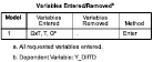
For econometric assessment of the impact of an openness policy (imports) in the intermediate inputs of the health industry on the difference between total and domestic effects, the following base regression is used (Pérez and Moral, 2015):

Y = a0 + a1G + a2T + a3G*T + e [1]

Y is the difference between total and domestic effects of the health sector on the whole national economy.

G is the dummy variable that distinguishes the group (treatment or control).

T is the dummy variable defining the baseline and the endline.

G x T is the interaction between the dummy variables G and T; its estimated coefficient is the value a3, statistical of difference in differences, which is that which assesses the impact of globalisation on the difference between total and domestic production multipliers.

56

The letter e represents the error term.

In addition, with the information provided by the ICIO database, we will analyse the modification of the imports structure in the health and social works sector. For the treatment of data and application of statistical techniques, SPSS software package (Statistical Package for Social Sciences) has been used.

Finally, we are interested in knowing the time trend of output multiplier gaps and trying to identify different profiles in the various geographical areas (EU15 and EU13) during the studied period 1995-2011. For that purpose we will utilise an econometric technique known as segmented regressions or joinpoint regression.

The trend analysis is based on series with few observations that have no noise, no seasonality, and only have a tendency. These types of studies are part of ecological, observational studies. Joinpoint is statistical program for the analysis of trends using joinpoint models, that is, models where several different lines are connected together at the “joinpoints”. The software takes trend data and fits the simplest joinpoint model that the data allow. The program starts with the minimum number of joinpoints (e.g. 0 joinpoints, which is a straight line) and tests whether more joinpoints are statistically significant and must be added to the model (up to that maximum number). This enables the user to test whether an apparent change in trend is statistically significant. The tests of significance use a Monte Carlo Permutation method. The models may also be linear on the log of the response (e.g. for calculating annual percentage rate change). The software also allows the viewing of one graph for each joinpoint model, from the model with the minimum number of joinpoints to the model with maximum number of joinpoints (Kim, et al., 2000).

57

2. Results

2.1 Descriptive data

The average value of the output multiplier in the health and social works sector for the 62 countries included in the OECD IOT was 1.8395 in 2011. This means that each additional monetary unit devoted to the final demand of this sector generates, directly and indirectly, an increase of 1.8395 dollars in the whole output of that national economy. This average value is much more reduced than those that we usually hear in politicians’ statements on the news, which are sometimes two or three times greater. In 1995 the average value of the output multiplier was 1.7733, so the increase was rather modest.

If we calculate the production multiplier without including imported inputs, we will have a different value for this multiplier. That new value reflects the “domestic” impact of one additional dollar spent for the final demand of one production sector on the whole “domestic” economy. This value remained almost invariable throughout 1995 (1.4791) and 2011 (1.4818). The most remarkable thing is the progressive growth of the distance between these two multipliers, the total and the domestic one.

In general, for the health and social works sector, differences between total and domestic production multipliers in 2011 are greater than in 1995. Considering the Rest of the World as the country number 62 in our sample, the previously mentioned differences increased in 73% of countries. And, that percentage increases to 79% when only OECD countries are taken into account. The differences between 2011 and 1995 values have been checked by means of the statistical T test. The T test confirmed the existence of a statistically significant difference between the multipliers gap in 1995 and 2011.

Within the group of OECD countries, the total production multiplier grew in 83% of cases between 1995 and 2011. For the same period, that growth can only be observed in 50% of cases for the domestic production multiplier. In addition, despite the total production multiplier being greater in 2011 than in 1995, the domestic production multiplier 58decreased between those two years in 13 OECD countries (e.g., USA, Spain, the Netherlands, Japan, Germany, etc.). This phenomenon is much less frequent in non-OECD countries. Regarding the differences among countries, the variation coefficient indicates greater dispersion among countries in 2011, although it is not relevant and is specifically concentrated in non-OECD countries.

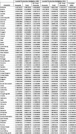
Table 1 reflects the multipliers gap for every country in 1995 and 2011 as well as the difference between both years. The growing value of the multipliers gap and, even more, the stagnant value of domestic multipliers during the studied period have a relevant implication for policy action. The continuous growth of healthcare expenses in most countries, both in absolute terms and in comparison with GDP, is one of the most prolonged phenomena in recent decades. Nevertheless, such a significant component of final demand has not been able to increase domestic multipliers at the same pace as total multipliers, thus the gap has become larger and larger.

Despite the traditional thought about healthcare expenditure presupposing strong backward and forward linkages in other industries, current evidence indicates that those linkages are not so strong, especially when only domestic effects are measured. The incorporation of new health technologies, expensive medicines, and diagnostic equipment, in medical practice and clinical guidelines, is one of the main drivers that explain why healthcare costs have increased so sharply in recent years.

In many countries, the chapter of healthcare expenses is mainly covered by public budgets, so that the direct and indirect impacts on other industries become a public policy issue. The observed stagnation of domestic multipliers in the health sector puts more emphasis on the importance of evaluating the cost-effectiveness of new health technologies before making a decision about their incorporation into medical practice and their coverage by public health systems.

59

Tab. 1 – Production Multipliers: Health and Social Work.

60

Once having ascertained the increasing gap between total and domestic multipliers (multipliers gap), we found some interesting associations of this phenomenon with the globalisation process. Two indicators can inform us about the degree of openness in national economies. The first one is a general indicator and refers to the whole economy, i.e., to the different economic activities. This is the so-called “Trade in goods and services” published by the OECD. One of the measures offered in that publication is the percentage of imports to the GDP. This measure is available for 40 countries, 34 OECD plus 6 non-OECD countries, from 1970 to 2015.

Moreover, we verified a clear positive association between the degree of commercial openness and the gap between production multipliers (total and domestic) for the Health and Social Works industry in 2011. This association could be considered weak, because it is comparing a global indicator with another that is very specific and exclusively related to one particular branch of activity. Notwithstanding, we need to associate the multipliers gap with a second indicator more specific and referring exclusively to the Health and Social Works services. This second indicator is the ratio of imports to intermediate inputs (intermediate consumptions) in the Health and Social Works sector. It shows the percentage of inputs that this production sector needs to buy abroad. A positive association between the ratio of imports to intermediate consumptions and the multipliers gap for most countries was also confirmed. The great heterogeneity among the group of countries included in the sample justifies the presence of outliers in both ratios, since we are including countries with a very different degree of development and social conditions. Nevertheless, as in general the share of imports in intermediate inputs has followed an increasing trend for most countries since 1995, we can intuitively think that this trend explains the growing multipliers gap.

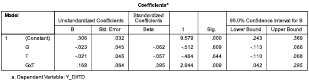
2.2 Difference in differences model

In order to test the causality of the relationship between the growth of imports share and the multipliers gap, we built a DiD econometric model. As this type of model requires the comparison of an experimental group with a control group, we have divided our sample with 62 61countries into two groups according to their share of imports in the total output of the Health and Social Works branch. Those countries with a share of imports greater than the median have been included in the experimental group. This group represents all countries that followed a commercial policy in favour of stronger foreign relationships and external trade. As external trade and commercial openness strengthen competitiveness, we have utilised total output as denominator instead of intermediate consumptions in the creation of the experimental and control groups.

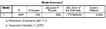
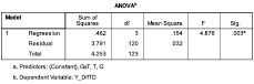
The results of the DiD model are shown in Table 2 and indicate that those countries that increased their imports share have also augmented their multipliers gap. Globally considered, the model fits the data well, with a significant value for the F test. In contrast, the sample autocorrelation of the residuals has been tested and the Durbin-Watson test, close to 2, indicates no autocorrelation. Finally, the most important thing in a DiD model is the statistical significance of the coefficient for the GxT variable. In this model, the sign is positive and the p value close to zero. Thus, we can say that those countries included in the experimental group have greater growths of multipliers gap.

For a better understanding of the results of the model, we must keep in mind that the DiD models do not intend to explain or anticipate a phenomenon by including all its determinant variables. For this reason, the coefficient of determination is usually very low compared to other econometric models. In this case, we can observe that R square is equal to 0.109. But we are not really interested in explaining the behaviour of the gap multipliers variable. We are simply concerned with demonstrating that growth of the multipliers gap for countries belonging to the experimental group was greater than that of the countries within the control group. The sign and statistical significance of G and T variables are not really important for our purpose. What is imperative for this work is the sign and statistical significance of the variable GxT, i.e. the combination of the group (experimental/control) and the time-period (initial/final). In Table 2 we can see the positive sign (+0.169) of B coefficient for GxT variable and its statistical significance (p value equal to 0.009). Both figures corroborate the hypothesis of greater increases for gap multipliers in those countries with a more pronounced commercial opening.

62

Tab. 2 – Difference in Differences Model Results.

Finally, we will look for reasons for these changes in multipliers gap. Concretely, we are going to study the share of each industry in the structure of intermediate consumptions and imports and how the shares have changed over the studied period.

The Health and Social Work industry has its intermediate inputs very concentrated in four specific industries: chemical products (C24); computer, electronic and optical equipment (C30-33); wholesale, retail trade, and repairs (C50-52); R&D and other business activities (C73-74). In 1995 these four activity branches concentrated 46% of intermediate consumptions and 68% of imports. In 2011 the relative importance of 63these four suppliers was equally relevant, 43% of intermediate inputs and 65% of imports.

From 1995 to 2011, two of these four activity branches gained importance in imports, chemical (pharmaceutical products) and R&D and other business activities (consultancy). Thus, the increase of resources devoted to those imports meant that the domestic output multiplier did not grow at the same pace as the total output multiplier.

Table 3 shows the contributions of each of the industries to the intermediate consumption of the health and social work industry (C85). These data are expressed in absolute terms (million US dollars) and in percentages over the total. Imported intermediate consumptions are also shown for 1995 and 2011. And finally, in the last two columns we can see the evolution of each industry’s share between 1995 and 2011 for total and imported intermediate consumptions.

Tab. 3 – Intermediate inputs and imports by industry.

64

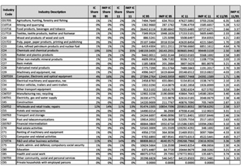
In general, we cannot say that the intermediate inputs structure suffered relevant changes between 1995 and 2011. Most industries show quite similar values of ‘share’ in both years. However, imports gained relevance in two of these main supplier industries.

In addition to the persistence of the high intensity in imports of the industries with a greater share in intermediate consumption, we have observed that industries with less relative weight as suppliers grew more intensively and more based on imports during the studied period. In absolute values, intermediate inputs in 2011 are equal to 2.85 times those of 1995, and imports in 2011 are 3.61 times greater than those of 1995. Nevertheless, 14 industries with a moderate relative size showed a growth rate higher than the average in intermediate inputs and imports as well.

2.3 Time trend analysis

The OECD database contains the TIOs for 61 countries, of which 34 belong to the OECD and 27 do not. Of these 27 non-OECD members, 7 are part of the EU13 (Bulgaria, Cyprus, Croatia, Lithuania, Latvia, Malta, and Romania). In 2011, the variability among output multipliers gap in the total set of countries is very high, with a variation coefficient reaching a value of 0.559. As we reduce the geographical scope of the analysis, the variability of the gaps is reduced. In the EU28 variability is notably reduced, leaving the coefficient equal to 0.335.

The differences in the year 2011 are still evident among the different groups of countries: EU15, EU13, OECD, and NON-OECD. The higher values are presented in the group of non-member countries of the OECD, although the EU13 group of countries offers the highest values within the OECD members. To obtain conclusions with respect to a more homogeneous economic environment we will restrict the trends analysis to EU countries, distinguishing between those that form part of the EU15 group and, those with the most recent membership, i.e., the EU13 group.

As Figure 1 shows, within the EU28, the differences between the EU15 and EU13 groups are notable and persist even at the end of the period analysed. The EU member states of recent incorporation show higher values in their multipliers gap, during the period studied. However, the differences between both groups lessened as the 1995-2011 65period elapsed, mainly due to the increase of the gap in the EU15 countries. This box-and-whisker diagram (box plot) presents one box for each group of countries in every year. Boxes for the EU13 have a greater dispersion and, while the median value maintains a relative stability throughout the studied period, the interquartile range has been progressively cut. In the EU15 group the evolution was quite stable with interquartile ranges that reflect a notable concentration of values. The increase of the median value has been very slight and the points representing Ireland and Luxemburg appear as outliers in the last three years. In summary, Figures 1 shows a progressive approximation of the median values of both groups of countries, which have grown since 2006.

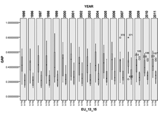
Fig. 1 – Trend of output multipliers gap in the EU.

Regarding the temporary evolution of multipliers gap, in the group EU15 all countries except Greece experienced growth between 1995 and 2011. However, in the group EU13 the proportion of countries with an increasing multipliers gap is much lower. Only 5 of the 13 countries that 66make up this group offer higher values in 2011 than in 1995. Even so, in the EU13 group most countries reached absolute values of multipliers gap notably higher than those of the EU15 countries.

Even within the EU, countries experienced different time trends throughout the period studied. These differences are specified in different rates of variation, different signs in evolution, and even variations of the opposite sign for multipliers gap in different subperiods.

The study of the dependent variable (multipliers gap) as a function of time (t) has been carried out applying the technique known as segmented regression or trend analysis. To accomplish it, we have used the Joinpoint software (National Cancer Institute, 2017). This software adjusts segmented regression models based on the annual percent change (APC). In the process the program looks for points of significant change in tendency. In this way, it is possible for us to have a function with several segments with different APC during the period studied. First, the program estimates a single linear function, with no change point. This first function is calculated by the mean square error, that is, the arithmetic mean of the squares of the errors (MSE0). Then the program repeats the estimate incorporating a single change point and recalculates MSE1. If MSE1 <MSE0, the second model will be preferred. It continues with a third model with 2 change points and recalculates MSE2. At the end, the program chooses the model that has the lowest MSE. The sequence of comparisons between models is based on a permutations test. Given the absence of significant differences, the program keeps the simplest model, that is, with which it has fewer points of change.

In the analysis of the time trend of the “multipliers gap” variable, we assume the hypothesis of normal distribution of errors, homoscedasticity, and the lack of correlation in the series. The results obtained for the EU15 group (Table 4) show a total of 7 countries in which the adjusted linear function does not indicate any cut-off point (joinpoint = 0) and the adjustment is statistically significant (p-value = 0): Denmark, France, Germany, Ireland, Italy, Portugal, and Sweden. The average APC for these seven countries is 3.1%. Denmark is the country with the highest APC (6.1%).

67

Tab. 4 – Annual Percentage of Change in EU15 multipliers gap.

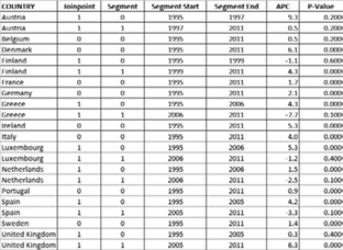
Four countries of the EU15 (Greece, Luxembourg, The Netherlands, and Spain) show adjustments with two segments and one joinpoint, in 2005 or 2006, which determines that the end of the first segment has a statistically significant increasing APC of 3.8%. The most important information obtained from Table 4 is that all the EU15 countries except Austria and Belgium have at least one period in which the adjusted linear function is statistically significant (p-value = 0) and the APC show a positive value. This finding reinforces the hypothesis about the homogeneity and the growing trend of the multipliers gap within the EU15 countries.

Figures 2 and 3 reflect the adjusted functions for Portugal and Spain, an example of countries where the trend offers 1 and 2 segments respectively with statistically significant adjustments. These different trends in two economies that were hit hard by the economic crisis of 2007 could be associated with different strategies in their foreign sectors. Although both countries experienced a large trade deficit during the years of the economic crisis, the recovery strategies were different. In the case of Portugal, trade balance was reached in 2012 and was based on a more 68pronounced growth in exports. Spain achieved trade balance in 2011, supported by a sharp decline in imports until 2009 and a subsequent growth of both flows, exports and imports, beginning this year. Given that the multipliers gap is linked to the intensity of imports, different commercial strategies in periods of deficit can give rise to different time trends in the short and medium term.

Fig. 2 – Time Trend and Annual Percent Change of Multiplier Gap
in Portugal 1995-2011.

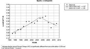
Fig. 3 – Time Trend and Annual Percent Change of Multiplier Gap
in Spain 1995-2011.

69

Most likely, if the analysed period were longer, the differences observed between the temporary trends of Spain and Portugal would disappear, since from 2011 both countries have continued a growth path in the flow of imports with respect to GDP. In any case, the implications derived from a decrease in the multipliers gap suggest a strengthening of the internal transmission, through direct and indirect effects, from the final demand to the national outputs.

By means of the trend parallelism test, we have analysed the existence of parallel trends among the countries of the EU15 group. The results reveal that the cases in which parallel trends are verified are relatively few and are concentrated in two countries, Portugal and Sweden, where the adjusted linear functions have no cut-off points. For each of these two countries it has been possible to adjust statistically significant parallel functions of five countries. Portugal maintains a parallel trend with those of Austria, Belgium, Germany, The Netherlands, and Sweden, while Sweden maintains parallel trend with those of France, Germany, Greece, Portugal, and Spain. The most relevant finding is that the two countries with the most parallel trends are countries with zero jointpoints and with a positive and statistically significant APC.

Figure 4 shows, as an example, the result of the comparison between Portugal and Sweden, with a statistically significant APC of 1.16%. As Sweden and Portugal are the countries in which the largest number of positive and statistically significant parallel trends were verified, this parallelism between them can be regarded as the synthesis image for EU15 countries.

70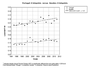

Fig. 4 – Parallel trend of multipliers gap between Portugal and Sweden.

The results obtained for the group EU13 (Table 5) show a total of 3 countries in which the adjusted linear function does not show any cut-off point (joinpoint = 0): Czech Republic, Slovenia, and Romania. But in this group, only the function adjusted for Romania with the APC being negative (-2.4%) is statistically significant.

71

Tab. 5 – Annual Percentage of Change in EU-13 multipliers gap.

Most of the countries in this group show irregular tendencies with 1 or 2 cut-off points that offer APC with positive and negative signs alternating over the period studied. In addition, in many cases the functions adjusted to the different segments are not statistically significant, which prevents solid conclusions. With respect to the existence of parallel trends among the countries of the EU13 group, results of the trend parallelism test showed that parallel trends were verified only for 10 countries, of which the parallel trends for 5 of them were produced in the comparison with Romania (Czech Republic, Estonia, Slovenia, Bulgaria, and Lithuania).

72

The comparison of both groups of countries reveals that the evolution of the multipliers gap has been considerably more stable in the group EU15, where the increasing trends predominate, some at times with a single segment and others with one joinpoint in 2005 or 2006. In contrast, in the EU13 group, trends have been much more irregular, with negative APC and segmented functions with one or two joinpoints in different years.

Conclusions

This work is based on the concept of multipliers gap, understood as the difference between the output multiplier obtained from the Leontief inverse matrix (total) and that obtained from the Leontief inverse matrix (domestic). Only 17 countries of the 62 included in the OECD database had multipliers gap in 2011 lesser than in 1995.

The main hypothesis was formulated as follows: “Globalisation and the change in the structure of imports in the health sector cause the total economic impact, which is derived from the growth in the final demand of this sector, to be progressively distancing itself from the impact on the domestic economy.” To measure these differences, we have assessed the distance between output multipliers– domestic and total. He term “Total” refers to the whole economy of a country, including imports and exports; while “Domestic” refers to a country’s economy, excluding imports and exports.

That hypothesis has two propositions. The first one affirms that, for the health sector, total and domestic output multipliers followed divergent trends during the period 1995-2011. The second one speculates on the cause of this divergent evolution and attributes that behaviour to globalisation and the structure of imports.

The first proposition was confirmed directly by descriptive data and by the T test. Both showed that the difference between output multipliers, domestic and total, became greater during the studied period. In general, domestic multipliers remained rather stable, while total multipliers presented increments greater than 6.6% or 8.3% in OECD countries.

73

The second proposition has been confirmed with the DiD econometric model and with the analysis of variations, industry by industry, in the inputs and imports structure of the health sector. The DiD model results demonstrated a positive causal relationship between imports intensity, as a proxy of globalisation, and multipliers gap. The industry by industry analysis showed a double influential shift towards the strengthening of imports in the health and social works industry. On the one hand, two of the most important supplier industries (chemicals and consultancy) have maintained their share in terms of inputs and imports. These two industries concentrate a high proportion of inputs and a high proportion of imports of the health sector. On the other hand, several industries with less relevance in terms of inputs have augmented notably their import shares.

The trend analysis showed that the EU15 countries have smaller but growing multipliers gap, while the EU13 countries have higher gaps, but their tendency is decreasing. Regarding the pattern of behaviour in the period studied, a certain homogeneity is observed in the EU15 group and a great variety among the countries of the EU13 group.

Two main limitations of this study must be stated. Both are related to the use of the input-output model. The first one is specifically related to the limitations of that model, derived from some assumptions of the input-output model which are related to the constancy of the input technical coefficients, the impossibility of factor substitution, and the considerations of final demand as an independent variable. The second limitation refers to the methodological difficulties of homogenising IOT elaborated with different national norms.

The lack of data from 2011 in the OECD IOT and the existence of three alternative inter-country input output databases complicate the continuity in the short term of this study even more. Nevertheless, a complementary line of study could be the extension of this analysis to the employment and value-added multipliers.

The most relevant contribution of this work is the verification of the initial hypothesis and the consequences derived from it. Once we have a general verification of the increase of output multipliers gap linked to globalisation and imported inputs for a sample with 62 countries, country by country specific analyses can be carried out with a combined use of the OECD IOT and ICIO databases. Trend analysis confirmed a quite similar pattern of behaviour in the EU15 countries.

74

It is important to take into account the double role played by globalisation. On the one hand, imported inputs have gained strength in national production structures, and certain patterns of specialisation along production chains can improve competitiveness. The increase in imports participation is consistent with recent studies published on the integration of national productive structures in global value chains. However, on the other hand, from the perspective of our analysis, the greater trade openness in the health sector coincides with generally stagnating domestic output multipliers that limit the direct and indirect domestic impacts of final demand for health services.

Finally, from the perspective of economic policy implications, the verification of the gap multipliers hypothesis reinforces the importance of a continuous surveillance of those multipliers in order to formulate realistic forecasts about the capacity of final demand (public and private) of healthcare services in boosting domestic output. Nonetheless, a key issue learned is that, despite the increasing multipliers gap, those countries with greater increments in total output multiplier also show the greatest positive variations in domestic output multipliers. Thus, economic policy should not go against globalisation and commercial opening-up.

75

References

Abbott P. A. and Coenen A. (2008), “Globalization and advances in information and communication technologies: The impact on nursing and health”, Nursing Outlook, 56(5), p. 238-246.

Aguiar A., Narayanan B., and McDougall R. (2016), “An Overview of the GTAP 9 Data Base”, Journal of Global Economic Analysis, 1(1), p. 181-208.

Angrist J.D. and Pischke J. (2009), Mostly Harmless Econometrics: An Empiricist’s Companion, Princeton University Press, Princeton, New Jersey: Princeton University Press.

Bess R., and Ambargis, Z. O. (2011), Input-Output Models for Impact Analysis: Suggestions for Practitioners Using RIMS II Multipliers, BEA Working Paper No. 81, Bureau of Economic Analysis.

Bettcher D. W., Yach D., and Guindon G. E. (2000), “Global trade and health: key linkages and future challenges”, Bulletin of the World Health Organization, 78(4), p. 521-534.

De Backer K. and Miroudot S. (2013), Mapping Global Value Chains, OECD Trade Policy Papers, Paris: Organisation for Economic Co-operation and Development.

Dollar D. and Kidder M., (2017), “Institutional Quality and Participation in Global Value Chains”, in World Bank, Global Value Chain Development Report: Measuring and Analyzing the Impact of GVCs on Economic Development. Washington, DC: World Bank, p. 161-173.

Gertler P. J., Martinez, S., Premand, P., Rawlings, L. B., & Vermeersch, C. M. J. (2011), “Impact Evaluation in Practice”. World Bank. Retrieved from https://openknowledge.worldbank.org/handle/10986/2550

Glinos I.A, (2015), “Health professional mobility in the European Union: Exploring the equity and efficiency of free movement”, Health Policy, vol. 119, nº 12, p. 1529-1536.

Haux R. (2006), “Individualization, globalization and health – about sustainable information technologies and the aim of medical informatics”, International Journal of Medical Informatics, 75(12), p. 795-808.

Hazarika I. (2010), “Medical tourism: its potential impact on the health workforce and health systems in India”, Health Policy and Planning, 25(3), p. 248-251.

Herman L. (2009), “Assessing International Trade in Healthcare Services”, SSRN Electronic Journal, http://doi.org/10.2139/ssrn.1395847

Hopkins L., Labonté R., Runnels V. and Packer C. (2010), “Medical 76tourism today: What is the state of existing knowledge?”, Journal of Public Health Policy, 31(2), p. 185-198.

Huynen M. M., Martens P., and Hilderink H. B. (2005), “The health impacts of globalisation: a conceptual framework”, Globalization and Health, 1, 14. https://doi.org/10.1186/1744-8603-1-14

IMS Institute for Healthcare Informatics (2016), Delivering on the Potential of Biosimilar Medicines: The Role of Functioning Competitive Markets. https://www.medicinesforeurope.com/wp-content/uploads/2016/03/IMS-Institute-Biosimilar-Report-March-2016-FINAL.pdf

Jones L., Wang Z., Xin L. and Degain C. (2014), The Similarities and Differences among Three Major Inter-Country Input-Output Databases and their Implications for Trade in Value-Added Estimates, Working Paper No. 2014-12B, Office of Economics U.S. International Trade Commission, Washington, DC 20436 USA.

Kim H.J., Fay M.P., Feuer E.J. and Midthune D.N. (2000), “Permutation tests for joinpoint regression with applications to cancer rates”, Stat Med, 2000, 19(3), p. 335-351.

Labonté R., Mohindra K. and Schrecker T. (2011), “The growing impact of globalization for health and public health practice”, Annual Review of Public Health, 32(1), p. 263-283.

Maier C. B. and Aiken L. H. (2016), “Expanding clinical roles for nurses to realign the global health workforce with population needs: a commentary”, Israel Journal of Health Policy Research, 5, 21.

Marchal B. and Kegels G. (2003), “Health workforce imbalances in times of globalization: brain drain or professional mobility?”, The International Journal of Health Planning and Management, 18(S1), p. S89-S101.

McMichael A. J. (2013), “Globalization, Climate Change, and Human Health”, New England Journal of Medicine, 368(14), p. 1335-1343.

Miroudot S., Lanz R. and Ragoussis A. (2009), Trade in Intermediate Goods and Services, OECD Trade Policy Papers, No. 93, OECD Publishing, Paris.

National Cancer Institute (2017), Joinpoint Regression Program, Version 4.5.0.0 - May 2017; Statistical Methodology and Applications Branch, Surveillance Research Program.

Pachanee, C. (2006), “Incoherent policies on universal coverage of health insurance and promotion of international trade in health services in Thailand”, Health Policy and Planning, 21(4), p. 310-318.

Pérez-López C. and Moral-Arce I. (2015), Técnicas de evaluación de impacto. Madrid, Spain: Garceta, Grupo Editorial.

Rana P. and Roy V. (2015), “Generic medicines: issues and relevance for global health”, Fundamental & Clinical Pharmacology, 29(6), p. 529-542.

77

Shaffer F. A., Bakhshi M., Dutka J. T. and Phillips J. (2016), “Code for ethical international recruitment practices: the CGFNS alliance case study”, Human Resources for Health, 14(Suppl 1), 31.

Smith R. D., Chanda R. and Tangcharoensathien V. (2009), “Trade in health-related services”, The Lancet, 373(9663), p. 593-601.

Timmer M. P., Dietzenbacher E., Los B., Stehrer R. and de Vries G. J. (2015), « An Illustrated User Guide to the World Input–Output Database: the Case of Global Automotive Production”, Review of International Economics, 23(3), p. 575-605.

Whittaker A., Manderson L. and Cartwright E. (2010), “Patients without Borders: Understanding Medical Travel”, Medical Anthropology, 29(4), p. 336-343.